38 how to wrap column labels in excel
Swimmer Plots in Excel - Peltier Tech 08.09.2014 · The first block of data is used to create the bands in the swimmer chart. Excel’s usual arrangement is to have X values in the first column of the data range and one or more columns of Y values to the right. Our data has Y values in the last column, and several columns of X values to the left. So putting this data into the chart will take a ... VBA Wrap Text (Cell, Range, and Entire Worksheet) - Excel Champs Use the following steps to apply Wrap Text using a VBA Code. Define the cell where you want to apply the wrap text using the range property. Type a dot to see the list of the properties and methods for that cell. Select the "WrapText" property from the list. Enter the equals sign "=" and the type TRUE to turn the wrap text ON.
Merge two excel files using a common column - Super User 10.12.2011 · I have placed the data from "the first excel" on Sheet1, and "the 2nd excel" on Sheet2. The key to this solution is the VLOOKUP() function. First we insert a column. We then use the VLOOKUP() function to lookup the value of "1" in Sheet2. We specify 2 as the value of the third parameter, meaning we want the value of the 2nd column in the array ...

How to wrap column labels in excel
How to wrap columns in Excel - Quora Answer (1 of 5): You can select non-contiguous columns by holding down the Ctrl key while selecting them. Then choose the Wrap command. In the following example Columns B, F, and L are selected. Select Wrap from the Format Cell dialog and the Alignment tab. This is the result. You can change t... Labeling Excel data groups - Microsoft Community If you want to filter columns by labels, you can select columns you want to name as a label, and set a name like test in the Name Box (on the left side of the command bar), then each time you type "test" in the Name Box, it will immediately place the cursor on the group you set up before like that: Meanwhile, if you have more ideas or ... How to wrap X axis labels in a chart in Excel? - ExtendOffice 1. Double click a label cell, and put the cursor at the place where you will break the label. 2. Add a hard return or carriages with pressing the Alt + Enter keys simultaneously. 3. Add hard returns to other label cells which you want the labels wrapped in the chart axis. Then you will see labels are wrapped automatically in the chart axis.
How to wrap column labels in excel. › filter-column-in-excelFilter Column in Excel (Example) | How To Filter a ... - EDUCBA Excel Column Filter (Table of Contents) Filter Column in Excel; How to Filter a Column in Excel? Filter Column in Excel. Filters in Excel are used for filtering the data by selecting the data type in the filter dropdown. By using a filter, we can make out the data that we want to see or on which we need to work. Excel tutorial: How to customize axis labels Now let's customize the actual labels. Let's say we want to label these batches using the letters A though F. You won't find controls for overwriting text labels in the Format Task pane. Instead you'll need to open up the Select Data window. Here you'll see the horizontal axis labels listed on the right. Click the edit button to access the ... How to Wrap Data to Multiple Columns in Excel - Excel Tips - MrExcel ... The FinalRow = line looks for the last entry in column 1. If your data started in column C instead of column A, you would change this: FinalRow = Cells (Rows.Count, 1).End (xlUp).Row. to this. FinalRow = Cells (Rows.Count, 3).End (xlUp).Row. In this example, the first place for the new data will be cell E2. › lock-column-in-excelHow To Lock a Column in Excel? - EDUCBA To lock a column in Excel, we first need to select the column we need to Lock. Then click right anywhere on the selected column and select the Format Cells option from the right-click menu list. Now from the Protection tab of Format Cells, check the box of LOCKED with a tick.
› charts › variance-clusteredActual vs Budget or Target Chart in Excel - Variance on ... Aug 19, 2013 · Set Data Labels to Cell Values Screenshot Excel 2003-2010. The nice part about either of these methods is that the data labels are linked to the values in the cells. If your numbers change or you update the data, the labels will automatically be refreshed and display the correct results. Please let me know if you have any questions. How to Wrap Text in Excel (In Easy Steps) Cell B1 is empty. 2. On the Home tab, in the Alignment group, click Wrap Text. 3. Click on the right border of the column A header and drag the separator to increase the column width. 4. Double click the bottom border of the row 1 header to automatically adjust the row height. Note: if you manually set a row height (by clicking on the bottom ... How to add total labels to stacked column chart in Excel? 1. Create the stacked column chart. Select the source data, and click Insert > Insert Column or Bar Chart > Stacked Column. 2. Select the stacked column chart, and click Kutools > Charts > Chart Tools > Add Sum Labels to Chart. Then all total labels are added to every data point in the stacked column chart immediately. Wrap Text in Excel - Top 4 Methods, Shortcut, How to Guide Method #3–Using the Keyboard Shortcut. The succeeding image shows a text string in cell A1. We want to wrap this string of cell A1. Use the keyboard shortcut Keyboard Shortcut An Excel shortcut is a technique of performing a manual task in a quicker way. read more for wrapping text.. The steps to wrap text in excel by using keyboard shortcut are listed as follows:
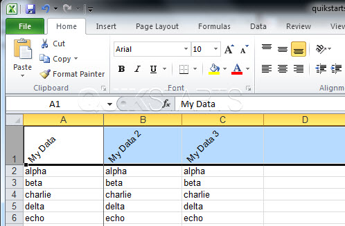
How to ☝️Wrap Text in Excel - SpreadsheetDaddy 1. Select one or more cells that you want to format. 2. Click the Home tab. 3. In the " Alignment" group, click the "Wrap text" button. Useful note: alternatively, you can use the Alt + H + W keyboard shortcut to do the same thing. Easy-peasy! We've reached our goal, and that's how the wrapped text looks like: Can't edit horizontal (catgegory) axis labels in excel - Super User 20.09.2019 · I FIGURED THIS OUT! It took me hours to figure this out. Hopefully, this will help someone else not spend hours on something so ridiculous.. I'm using Excel 2013. Like in the question above, when I chose Select Data from the chart's right-click menu, I could not edit the horizontal axis labels!. I got around it by first creating a 2-D column plot with my data. Edit titles or data labels in a chart - support.microsoft.com To edit the contents of a title, click the chart or axis title that you want to change. To edit the contents of a data label, click two times on the data label that you want to change. The first click selects the data labels for the whole data series, and the second click selects the individual data label. Click again to place the title or data ... How to wrap text in column headings in Excel I can wrap the text in the column headings, so the focus is on the contents in the cell, not on the width of the column. I select the entire row A1, and right click. I then select format cells, and click Wrap Text. Under Text alignment, select the Vertical text box and select Top. Format cells options. Now, for each column I can amend the ...
Displaying Column Charts with Long Label Names | SAP Blogs
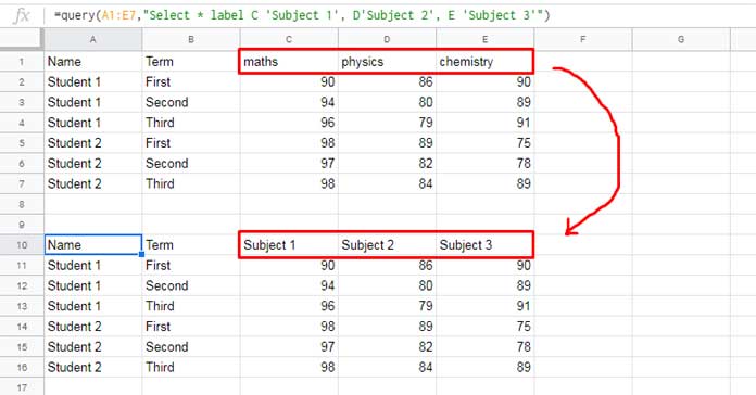
Comparison Chart in Excel | Adding Multiple Series Under Same … Now, if you see at the right-hand side, there is a Horizontal (Category) Axis Labels section. This is the one where you need to edit the default labels so that we can segregate the sales values column Country wise. Step 8: Click on the Edit button under the Horizontal (Category) Axis Labels section. A new window will pop up with the name Axis ...

30 How To Label Columns In Excel - Labels For You
Carriage Return in Excel Formula to Concatenate (6 Examples) 24.05.2022 · Method 5: VBA Macro Custom Function to Join the Entries with Carriage Return. Excel VBA Macros are very efficient in achieving desired outcomes. In this method, we demonstrate a custom function generated by a VBA Macro Code to insert a carriage return within a concatenated text string. Therefore, we slightly modify the dataset combining Name and …
Excel 2007's Wrap Text command makes formatting cells a snap - TechRepublic
excel Flashcards | Quizlet Study with Quizlet and memorize flashcards terms like An excel file that contains one or more worksheets., The primary document that you use in excel to store and work data, and which is formatted as a pattern of uniformly spaced horizontal and vertical., Another name for …

r - How to order X axis labels using facet_wrap() - Stack Overflow
How To Wrap Text In Excel - (2 Easy Ways + Shortcut) Here are the steps: Select the cell (s) for word wrapping. We will select column B. Right-click the selected cells. Select Format Cells from the context menu to launch the Format Cells dialog box (or use the keyboard shortcut Ctrl + 1 or click the dialog launcher arrow in the Alignment group under the Home ).

Custom Lists in Excel | Custom, Custom ribbon, Excel
MS Excel 2016: How to Create a Pivot Table - TechOnTheNet Finally, we want the title in cell A1 to show as "Order ID" instead of "Row Labels". To do this, select cell A1 and type Order ID. To do this, select cell A1 and type Order ID. Your pivot table should now display the total quantity for each Order ID as follows:

Counting Labels Without Numbers In Excel
How to Print Labels from Excel - Lifewire Select Mailings > Write & Insert Fields > Update Labels . Once you have the Excel spreadsheet and the Word document set up, you can merge the information and print your labels. Click Finish & Merge in the Finish group on the Mailings tab. Click Edit Individual Documents to preview how your printed labels will appear. Select All > OK .

Power of Excel: Transpose data from rows to columns, or vice versa
Wrap text in a cell - support.microsoft.com Adjust the row height to make all wrapped text visible. Select the cell or range for which you want to adjust the row height. On the Home tab, in the Cells group, click Format. Under Cell Size, do one of the following: To automatically adjust the row height, click AutoFit Row Height. To specify a row height, click Row Height, and then type the ...
How to Set Row Label Width in Excel 2010 | Daves Computer Tips
How to Wrap Text in Microsoft Excel To do so, select the cell you want to type in while wrapping. Navigate up to the formula bar just below the ribbon and click it. Begin typing. When you reach the end of the line you wish to wrap, position your cursor at the end of the line and press Alt+Enter. This will neatly wrap the text in the cell.

Counting Labels Without Numbers In Excel
› wp-content › uploadsUsing Excel for Analyzing Survey Questionnaires - WCASA To begin creating your Excel database: Type the survey title in the first cell at Row 1, Column A(“Type your title here” in Figure 2, “Title of survey” in Figure 3). Then move down two rows to Row 3, Column A. This is where you will enter column headers — labels to identify each question in your survey. Create column headers
6
How to wrap text in Excel automatically and manually - Ablebits Method 1. Go to the Home tab > Alignment group, and click the Wrap Text button: Method 2. Press Ctrl + 1 to open the Format Cells dialog (or right-click the selected cells and then click Format Cells… ), switch to the Alignment tab, select the Wrap Text checkbox, and click OK. Compared to the first method, this one takes a couple of extra ...

31 Create Label In Excel - Labels For Your Ideas
4 Ways to Wrap Text in Excel | How To Excel Select the cells from which you want to remove the formatting and then perform any of these methods. Go to the Home tab and press the Wrap Text command. Open the Format Cells menu and uncheck the Wrap text option in the Alignment tab. Use the Alt H W keyboard shortcut. The exact same commands used to apply the formatting can be used to remove ...
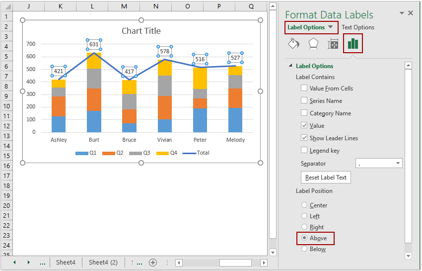
How to add total labels to stacked column chart in Excel?
superuser.com › questions › 366647Merge two excel files using a common column - Super User Dec 10, 2011 · I have placed the data from "the first excel" on Sheet1, and "the 2nd excel" on Sheet2. The key to this solution is the VLOOKUP() function. First we insert a column. We then use the VLOOKUP() function to lookup the value of "1" in Sheet2. We specify 2 as the value of the third parameter, meaning we want the value of the 2nd column in the array.
29 Label Columns In Excel - 1000+ Labels Ideas
How To Filter a Column in Excel? - EDUCBA For applying Excel Column Filter, select the top row first, and the filter will be applied to the selected row only, as shown below. Sometimes when we work for a large set of data and select the filter directly, the current look of the sheet can be applied.
34 How To Label Series In Google Sheets - Labels 2021
Text Labels on a Vertical Column Chart in Excel - Peltier Tech In Excel 2003 go to the Chart menu, choose Chart Options, and check the Category (X) Axis checkmark. Now the chart has four axes. We want the Rating labels at the left side of the chart, and we'll place the numerical axis at the right before we hide it. In turn, select the bottom and top vertical axes. In the Excel 2007 Format Axis dialog ...

How to edit the label of a chart in Excel? - Stack Overflow
superuser.com › questions › 1484623Can't edit horizontal (catgegory) axis labels in excel Sep 20, 2019 · I'm using Excel 2013. Like in the question above, when I chose Select Data from the chart's right-click menu, I could not edit the horizontal axis labels! I got around it by first creating a 2-D column plot with my data. Next, from the chart's right-click menu: Change Chart Type. I changed it to line (or whatever you want).
31 How To Label Excel Columns - Labels Database 2020
Actual vs Budget or Target Chart in Excel - Variance on Clustered ... 19.08.2013 · The file below uses a slightly different technique by using a clustered column chart to display the variance, and then uses the Value from Cells option to display the data labels. This only works in Excel 2013. The advantage is that you can automatically display the variance label above the bar, and you don't have to move it manually as the numbers change.

35 Select Max Label - Labels For Your Ideas
How to wrap column labels of calculated fields in a pivot table I created a Pivot Table using calculated fields (columns C-F). I am trying to wrap the text in the labels, but when I click into the cell, it just brings up a pop-up window, and I am unable to modify the formatting of the text. However, for the labels of non-calculated fields (A-B), I am able to modify the text format just fine.

31 How To Label Columns In Excel - Labels Database 2020
Using Excel's Wrap Text Feature - YouTube Oftentimes in Excel, users have text labels that do not fit neatly into a single column. Typically, they attempt to solve this problem by either increasing t...
Post a Comment for "38 how to wrap column labels in excel"